# Bandwidth
Capture the same current pulse twice, once at the full 1 Msps sample rate
and once at 50 ksps with the sinc3 filter. The first capture shows a narrow
30 mA spike. The second shows a wider bump that peaks near 10 mA. Which one
is right?
Both are. Each capture shows the same current, viewed through a different
bandwidth. Lower bandwidth spreads a short event out in time, which lowers
its peak, but the charge and energy of the event stay the same. This page
explains why, and what limits the bandwidth of a real measurement.
#### TIP
When you report a peak current, also report the sample rate and filter
used to measure it. A peak without a bandwidth is not a complete
measurement. Average current, charge and energy do not depend on the
bandwidth.
## What bandwidth means
Any waveform can be described as a sum of sine waves at different
frequencies. Slow changes need only low frequencies. Sharp edges and short
pulses also need high frequencies.
Every measurement passes the signal through a low-pass filter, whether by
design or not. The filter passes low frequencies and attenuates high ones.
Its *bandwidth* is the frequency at which the gain falls to −3 dB, about
71 % of the input amplitude. Above the bandwidth, the measurement
increasingly loses the high-frequency content of the signal.
Remove the high frequencies from a short pulse and the pulse can no longer
be short. Its energy spreads out over a longer time, so its peak drops. A
useful rule of thumb relates the bandwidth *BW* to the fastest rise time
*tr* (10 % to 90 %) that a measurement can show:
$$
t_r \approx \frac{0.35}{BW}
$$
A 300 kHz measurement shows edges as fast as about 1.2 µs. A 13 kHz
measurement cannot show anything faster than about 27 µs. A pulse much
shorter than *tr* appears with a width of about *tr* and a
peak reduced in proportion.
The filters used for measurement have a DC gain of exactly one. They move
charge around in time, but never add or remove it. The area under the
current waveform, the charge, is the same at every bandwidth. Like a pile of
sand that is raked flat, the pile gets wider and lower, but the amount of
sand does not change.
## Sample rate and bandwidth
Sample rate and bandwidth are related, but they are not the same thing. A
sampled signal can only represent frequencies below half the sample rate,
called the Nyquist frequency. Any content above it aliases, or folds back,
to a lower frequency where it corrupts the measurement. So, before reducing
the sample rate, an instrument must first filter away the content that the
lower rate cannot represent. This filter sets the bandwidth at the new rate.
Joulescope instruments downsample with sinc filters, also called moving
average or boxcar filters. A sinc1 filter averages each group of input
samples into one output sample. Going from 1 Msps to 50 ksps averages 20
samples. A sinc2 filter applies the average twice, and a sinc3 filter three
times. Each additional stage rejects more of the aliased content and gives
a smoother result, at the cost of lower bandwidth and a longer time window:
a sinc3 filter at 50 ksps combines input samples from a window about 60 µs
long.
| Filter | Bandwidth (−3 dB) | At 50 ksps |
|----------|---------------------|--------------|
| sinc1 | 0.443 × output rate | 22 kHz |
| sinc2 | 0.319 × output rate | 16 kHz |
| sinc3 | 0.262 × output rate | 13 kHz |
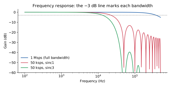
Frequency response at 1 Msps and at 50 ksps with sinc1 and sinc3
filters. Each curve’s bandwidth is where it crosses the dashed −3 dB line.
For the filters available on each instrument, and the analog bandwidth at the
full sample rate, see the Filters and Frequency Response chapter of your
instrument’s user’s guide, for example [the JS320 User’s Guide](https://docs.joulescope.com/en/products/js320/guide/filters.md#js320-filters-and-frequency-response) or [the JS220 User’s Guide](https://docs.joulescope.com/en/products/js220/guide/filters.md#js220-filters-and-frequency-response).
## Example: one pulse, multiple views
[Fig. 2](#theory-bandwidth-pulse-figure) shows a simulated 10 µs, 30 mA current
pulse on a 1 mA baseline, measured at 1 Msps and at 50 ksps, 10 ksps and
1 ksps with sinc1 and sinc3 filters.
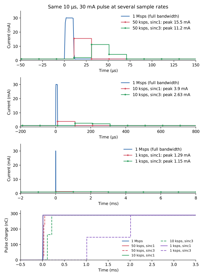
Top three plots: the same pulse at 1 Msps, and at 50 ksps, 10 ksps and
1 ksps with sinc1 and sinc3 filters. Note the different time scales.
Bottom: the charge of the pulse, which reaches 290 nC in every case.
| Sample rate | Filter | Peak shown | Peak range | Charge |
|---------------|----------|--------------|-----------------|----------|
| 1 Msps | none | 30 mA | 30 mA | 290 nC |
| 50 ksps | sinc1 | 15.5 mA | 8.4 to 15.5 mA | 290 nC |
| 50 ksps | sinc3 | 11.2 mA | 8.2 to 11.6 mA | 290 nC |
| 10 ksps | sinc1 | 3.9 mA | 2.5 to 3.9 mA | 290 nC |
| 10 ksps | sinc3 | 2.6 mA | 2.5 to 3.2 mA | 290 nC |
| 1 ksps | sinc1 | 1.29 mA | 1.15 to 1.29 mA | 290 nC |
| 1 ksps | sinc3 | 1.15 mA | 1.15 to 1.22 mA | 290 nC |
* At 1 Msps, the pulse is wider than the measurement rise time, so the
measurement shows its full 30 mA peak.
* A sinc1 filter reports the average current over each output sample. When
the pulse lands inside one sample, that sample shows the baseline plus the
pulse averaged over the sample period: 15.5 mA over 20 µs at 50 ksps,
3.9 mA over 100 µs at 10 ksps, and 1.29 mA over 1 ms at 1 ksps.
* A sinc3 filter spreads the pulse over three output samples, so its peak is
lower still.
* At 1 ksps, the pulse barely rises above the 1 mA baseline. The pulse is
still there: its charge is in the measurement, spread over a few
milliseconds.
The charge of the pulse, the lower plot, is 290 nC in every view. The
1 Msps view shows when the charge flowed in more detail. The lower rates
only show that it flowed within one to three output samples.
The reduced peak also depends on where the pulse falls relative to the
output sample boundaries, shown as the peak range in the table. The plots
show the alignment with the highest sinc1 peak. Repeated captures of
identical events can therefore show different peaks at a low sample rate.
At 1 Msps the peak stays at 30 mA, because the pulse is wider than the
measurement rise time.
The same effect applies at the full sample rate to pulses that are shorter
than the instrument’s rise time. A 300 ns spike appears at full rate as a
lower, wider pulse a few microseconds long.
## Choosing a sample rate
Choose the sample rate and filter for the quantity you need:
Peak current
: Use the full sample rate. Peak current matters when sizing a power
supply or regulator, choosing a battery for its internal resistance, or
looking for brown-out conditions. Even at full rate, check that the event
is longer than a few microseconds; see
[Measurement bandwidth](#theory-bandwidth-measurement).
Average current, charge and energy
: Any sample rate works. Lower sample rates reduce file sizes and USB
traffic for long captures, such as battery life estimates. To measure the
charge or energy of a single event, place x-axis dual markers around it in
the Joulescope UI’s Oscilloscope View. The result is the same at every
sample rate, as long as the markers include the whole event.
Comparing captures
: Use the same sample rate and filter for every capture you compare, and
compare peaks only between captures with the same bandwidth.
Lower sample rate without spreading
: Prefer sinc1. At 50 ksps, its 20 µs window spreads events the least.
Prefer sinc3 when you want a smoother waveform with less aliased noise,
and the peak of short events does not matter.
## Measurement bandwidth
The *measurement bandwidth* is the bandwidth of the instrument itself. It
combines:
* the analog front end, which includes the amplifiers and an anti-aliasing
filter before the analog-to-digital converter,
* any digital filter on the instrument or in the host software, and
* the downsampling filter for the sample rate you choose.
Joulescope instruments have a measurement bandwidth of a few hundred kHz at
the full sample rate. The exact values are in each instrument’s
specifications. The measurement bandwidth is an upper limit: no setting can
show detail faster than it. However, it is often not the limit that matters.
The circuit around the instrument usually limits the bandwidth first.
## System bandwidth
The *system bandwidth* is the bandwidth of everything between the current
you want to know and the number on your screen. It includes the measurement
bandwidth, but also your circuit.
Most products have capacitors on their supply input, and a Joulescope
measures current through a shunt resistor in series with the supply. Together
they form an RC low-pass filter, shown in [Fig. 3](#theory-bandwidth-system-figure).
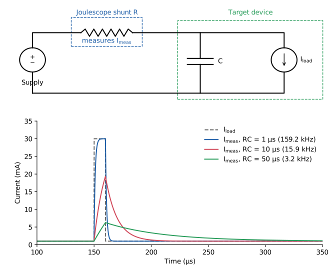
Top: the target’s input capacitance C and the Joulescope shunt resistance
R form a low-pass filter. Bottom: current that the Joulescope measures for
a 10 µs, 30 mA load pulse, for three RC time constants.
When the load inside the target draws a sudden pulse of current, the nearby
capacitor supplies it first. The capacitor’s voltage drops slightly, and
current then flows through the shunt resistor to recharge it. The
Joulescope measures that recharge current. The current through the shunt
follows the load current through a filter with time constant τ and
bandwidth *fc*:
$$
\tau = R \, C, \qquad f_c = \frac{1}{2 \pi R C}
$$
Here *R* is the total resistance between the supply and the capacitor: the
active shunt resistor, plus the cables, connectors and the supply’s output
impedance. *C* is the total capacitance on the target’s supply input.
Joulescope selects the shunt resistor based on the present current, keeping
the voltage across it small; see the Theory of operation chapter of your
instrument’s user’s guide, for example [the JS320 User’s Guide](https://docs.joulescope.com/en/products/js320/guide/theory.md#js320-theory-of-operation). The shunt resistance is small on the high
current ranges and large on the low current ranges, so the system bandwidth
changes with the current range. With C = 10 µF:
| Shunt resistance | τ = RC | System bandwidth |
|--------------------|----------|--------------------------------------|
| 0.01 Ω | 0.1 µs | Limited by cables and supply instead |
| 1.1 Ω | 11 µs | 14 kHz |
| 111 Ω | 1.1 ms | 140 Hz |
Autoranging helps. When a pulse arrives, the voltage across the shunt
rises, and the Joulescope switches to a lower resistance within about 1 µs.
This raises the system bandwidth for the rest of the pulse. Small pulses
that stay within the present range still see the full shunt resistance.
When several filters are in series, the combined rise time is approximately
the square root of the sum of the squares of the individual rise times. The
slowest one dominates. A 1 µs pulse measured by a 300 kHz instrument
through a 14 kHz RC filter is limited by the RC filter, and increasing the
sample rate does not change that.
Just as with sample rate, the RC filter does not change the charge. All of
the charge that the load draws eventually flows through the Joulescope to
recharge the capacitor, so average current, charge and energy remain
accurate.
### What you are measuring
With capacitance on the target, the Joulescope measures the current that the
target draws from its supply, not the current inside the target. For
battery-powered products, this is usually exactly what you want: the
battery also sees the current filtered by the capacitor.
To see the load current inside the target, reduce the capacitance between
the Joulescope and the load. You can move bulk capacitors to the supply side
of the Joulescope, or measure at a point after the capacitors, such as the
output of a regulator. Keep in mind that changing the capacitance changes
how the target behaves. Too little capacitance can cause the supply
voltage to sag during load pulses.
Regulators inside the target, such as LDOs and switching converters, also
shape the current. A switching converter draws input current in pulses at
its switching frequency, and its input capacitor smooths them in the same
way.
## Summary
* Bandwidth limits how fast a measurement can change. Short events appear
wider and lower at lower bandwidth.
* Charge and energy do not depend on bandwidth.
* Lower sample rates use filters with lower bandwidth. Higher order sinc
filters reduce the bandwidth further.
* The measurement bandwidth is the instrument’s limit. The system bandwidth
includes your circuit, and the shunt resistance together with the target’s
capacitance often limits it first.
* Report peak current together with the sample rate and filter.