# Efficiency
A power converter, such as a DC-DC regulator, an LDO or a battery charger,
delivers less power than it draws. Its efficiency is the fraction of the
input power that reaches the output:
$$
\eta = \frac{P_{OUT}}{P_{IN}}
$$
Efficiency changes with the load. A converter that is 92% efficient at
100 mA may be 60% efficient at 100 µA, where its own quiescent current
dominates. Battery-powered products spend most of their time at light load,
so the efficiency at the load your product actually draws matters more than
the peak value in the converter datasheet.
Measuring efficiency takes two instruments: one on the converter input and
one on the output. This page explains how to connect them so that the
instruments do not affect the result, how to check the setup, and what
limits the accuracy. The Joulescope UI computes efficiency with the
[Efficiency widget](https://docs.joulescope.com/en/software/joulescope_ui/widgets/efficiency.md#ui-efficiency).
## Wiring that removes burden voltage
Every ammeter adds a small voltage drop, called the burden voltage, across
its current path. If a voltmeter measures on the wrong side of an ammeter,
the burden voltage becomes part of the measured power, and the efficiency
reads wrong. For example, a 20 mV drop on a 3.3 V output changes the
measured output power, and the efficiency, by 0.6%.
Connect each Joulescope so that its voltmeter measures at the converter
pins, as shown in [Fig. 7](#theory-efficiency-wiring-figure):
* **Input Joulescope**: the current path goes from the supply to the
converter input. Connect **Voltage +** and **Voltage -** to the converter
VIN and GND pins, after the Joulescope.
* **Output Joulescope**: the current path goes from the converter output to
the load. Connect **Voltage +** and **Voltage -** to the converter VOUT
and GND pins, before the Joulescope.
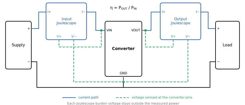
Efficiency wiring with each voltmeter connected at the converter pins.
Each Joulescope then measures exactly the converter’s input or output
current, and the voltage at the converter’s own pins. The burden voltage of
the input Joulescope lowers the voltage that the supply delivers to the
converter, and the burden voltage of the output Joulescope lowers the
voltage at the load. Both change the operating point slightly, but neither
appears in the measured power, so neither affects the measured efficiency.
Connect the voltage wires right at the converter pins, separate from the
current wires. Current through a shared wire or connector causes its own
voltage drop, just like the burden voltage. This is a Kelvin, or 4-wire,
connection.
### Instrument support
The JS220 and JS320 have separate **Voltage +** and **Voltage -** inputs,
so they work as either the input or the output instrument. Their sensor
side is isolated from the host computer, so you can place their current path
on either the positive (high side) or the ground (low side) connection.
The JS110 voltmeter measures between **IN+** and **IN-**, before its
current shunt (see the [JS110 Theory of operation](https://docs.joulescope.com/en/products/js110/guide/theory.md#js110-theory-of-operation)). Connect the JS110 with its IN terminals at
the converter output, and it works as the output instrument. Keep those
wires short, since the JS110 has no separate voltage wires to the converter
pins. As the input instrument, its own burden voltage is included in the
input power, and the efficiency reads slightly low.
The converter input and output usually share a ground. Since the
instruments are isolated, they do not add a ground connection of their own,
but other equipment can. See [Ground loops](https://docs.joulescope.com/en/theory/ground_loops.md).
## Check the setup before you measure
Two simple substitutes for the converter check the wiring, the instrument
assignment and the software before you measure the real converter.
**Null test.** Replace the converter with a wire, so that both instruments
measure the same current and the same node voltage. The efficiency must
read 100%, within the instruments’ accuracy. A JS220 and a JS320 in series,
for example, read 99.98%. A reading well above 100% usually means that the
input and output instruments are swapped.
**Resistor test.** Replace the converter with a series resistor R, and use
a resistive load RL. The input and output currents are equal, so the
efficiency is the ratio of the voltages:
$$
\eta = \frac{V_{OUT}}{V_{IN}} = \frac{R_L}{R + R_L}
$$
Change RL and check that the efficiency follows.
## Accuracy
The efficiency error is about the sum of the power errors of the two
instruments. At moderate loads the gain errors dominate. At light load,
the current offset of each instrument becomes a larger fraction of the
measured current, and it dominates. See the datasheet of each instrument,
available from [Products](https://docs.joulescope.com/en/products/index.md), for the current and voltage accuracy
in each range.
A converter in a light-load mode, often called burst, skip or PFM mode,
switches in bursts with long idle periods between them. Its input and
output current are pulses on a small average. Measure over a window that
contains many bursts so that the average is stable.
## Two instruments, two clocks
Each instrument has its own sample clock. The clocks run at slightly
different rates, and each instrument reports statistics on its own schedule.
Dividing one instrument’s statistics by the other’s pairs two different
time windows. When the load changes, the two windows contain different
amounts of energy, and the result is wrong.
The fix is to integrate the input power and the output power over the same
time interval. The host computer maps each instrument’s samples to UTC time
and corrects for the clock rate difference. The energy over a common
interval then comes from each instrument’s samples, and the efficiency is
the ratio of the two energies.
The time mapping is not perfect. A JS220 and a JS320 on the same computer
stayed aligned within about ±160 µs. For a steady load, this residual has
no effect. For a load step inside the measurement window, the error is
roughly the misalignment divided by the window duration: about 0.03% for a
0.5 s window, and about 1.6% for a 10 ms window. Use a longer window when
the load changes often.
## Energy storage in the converter
A converter has capacitors on its input and output, and switching
converters also have an inductor. These store energy. When the load
increases, the output capacitor delivers energy before the input supplies
it, and when the load decreases, the capacitors recharge.
Over a short window that contains a load change, the measured efficiency can
swing low or even exceed 100%. This is a real measurement of the energy that
flowed in that window, but it is not the converter’s efficiency. Measure
efficiency over windows where the load is steady, or over a long period that
contains many load changes. The cumulative efficiency, the total output
energy divided by the total input energy, is the right number for a
product that cycles between activity and sleep.
## Efficiency vs load
A converter datasheet plots efficiency against output current, usually on a
logarithmic current axis. To measure the same curve, hold the load at a
series of levels, and measure the efficiency at each.
You do not need a programmable load or a fixed sweep. The Joulescope UI
builds the curve from whatever loads your product draws:
* It measures the efficiency of each window, as described above.
* It keeps only steady windows, where neither the input nor the output
power changes by more than a small fraction within the window. This
excludes load changes and the energy storage they cause.
* It groups the steady windows into logarithmically spaced load bins. Each
bin’s efficiency is its total output energy divided by its total input
energy, so that a few noisy windows do not bias the result.
Dwell at each load for at least several windows. A load that changes
faster than the window produces no steady windows, and so no curve points.